画像のビニング(Binning)は、おそらく多くの方にとって聞き慣れない用語かもしれません。しかし、この概念はデジタルイメージング、特にデジタルカメラや顕微鏡、さらには自動車の運転支援システムなど、多くの技術分野で非常に重要です。簡単に言うと、ビニングは画像の解像度を下げることで、その他の画像品質(例:明るさ、ノイズの低減)を改善する手法です。
[ad]
ビニングとは何か
ビニングとは、隣接するピクセル(画像を構成する最小単位)をまとめて、一つの新しいピクセルとして扱うことです。例えば、2×2のビニングでは、2×2のピクセルブロックが一つの新しいピクセルにまとめられます。これにより、画像の解像度は下がりますが、その代わりに各ピクセルが持つ情報(光量など)が増加します。
Pythonでの実装
import numpy as np
import matplotlib.pyplot as plt
from PIL import Image, ImageSequence, ImageChops
from scipy.stats import norm
import os

def bin_image(image, bin_size):
    rows, cols = image.shape
    binned_rows = rows // bin_size[0]
    binned_cols = cols // bin_size[1]
    binned_image = np.zeros((binned_rows, binned_cols))
    for i in range(0, binned_rows * bin_size[0], bin_size[0]):
        for j in range(0, binned_cols * bin_size[1], bin_size[1]):
            block = image[i:i + bin_size[0], j:j + bin_size[1]]
            binned_image[i // bin_size[0], j // bin_size[1]] = np.mean(block)
    return binned_image

def plot_histogram_and_get_std(data1, data2, title1, title2):
    plt.hist(data1.ravel(), bins=256, range=(0, 256), color='gray', density=True, alpha=0.5, label=title1)
    plt.hist(data2.ravel(), bins=256, range=(0, 256), color='blue', density=True, alpha=0.5, label=title2)
    plt.title(f'Overlayed Histograms - {title1} & {title2}')
    plt.xlabel('Pixel Value')
    plt.ylabel('Frequency')
    plt.grid(True)
    plt.legend(loc='upper right')
    mu1, std_dev1 = norm.fit(data1.ravel())
    mu2, std_dev2 = norm.fit(data2.ravel())
    return std_dev1, std_dev2

def save_images_as_tif(images, save_path):
    images[0].save(save_path, save_all=True, append_images=images[1:])

# Load the image
image_path = 'image_name_here.jpg'  # Replace with your actual image path
original_image = Image.open(image_path).convert('L')
original_image_array = np.array(original_image)

# Perform binning at multiple bin sizes
bin_sizes = [(2, 2), (4, 4), (8, 8)]
std_dev_results = {}
collected_images = []
collected_histograms = []

for size in bin_sizes:
    binned_image_array = bin_image(original_image_array, size)
    binned_image = Image.fromarray(np.uint8(binned_image_array))
    collected_images.append(binned_image)

    plt.figure(figsize=(6, 6))
    std_dev_original, std_dev_binned = plot_histogram_and_get_std(original_image_array, binned_image_array, f'Original - Bin Size: {size}', f'Binned - Bin Size: {size}')
    histogram_image_path = f'histogram_{size[0]}x{size[1]}.png'
    plt.savefig(histogram_image_path)
    plt.close()  # Close the plot after saving
    histogram_image = Image.open(histogram_image_path).convert('L')
    collected_histograms.append(histogram_image)

    std_dev_results[size] = (std_dev_original, std_dev_binned)

# Save images and histograms as multi-page TIF files
collected_images_tif_path = os.path.splitext(image_path)[0] + '_collected_images.tif'
collected_histograms_tif_path = os.path.splitext(image_path)[0] + '_collected_histograms.tif'
save_images_as_tif(collected_images, collected_images_tif_path)
save_images_as_tif(collected_histograms, collected_histograms_tif_path)

# Save the standard deviations to a text file with the same name as the input image
output_file_path = os.path.splitext(image_path)[0] + '_multi_bin_std_dev.txt'
with open(output_file_path, 'w') as f:
    for size, (std_o, std_b) in std_dev_results.items():
        f.write(f"Bin Size: {size}\n")
        f.write(f"Standard Deviation of Original Image: {std_o}\n")
        f.write(f"Standard Deviation of Binned Image: {std_b}\n\n")
上記のプログラムは、Pythonを使用して画像のビニングを行う簡単な例です。このプログラムでは、NumPyとMatplotlibというライブラリを使用しています。NumPyは数値計算を高速で行うためのライブラリであり、Matplotlibはデータを視覚的に表示するためのライブラリです。
コードの主要部分について
- bin_image関数: この関数は、与えられた2Dの画像(NumPy配列)とビニングサイズ(例:2×2)を受け取り、ビニング処理を行った後の新しい画像を返します。
- 画像の生成: 10×10のサイズでランダムなグレースケール値(0~255)を持つサンプル画像を生成しています。
- ビニングの実行: bin_image関数を呼び出して、2×2のビニングサイズでビニング処理を行います。
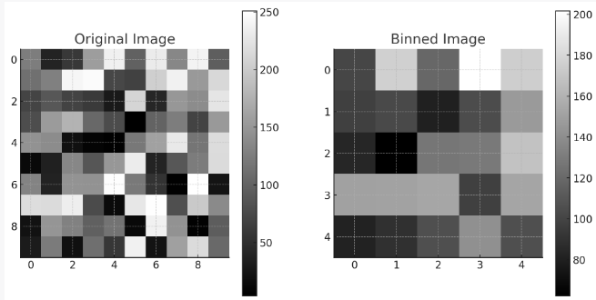
- 結果の表示: オリジナルの画像とビニング後の画像を並べて表示しています。
左側がオリジナルの10×10の画像、右側が2×2のビニング処理を行った後の5×5の画像です。色の濃淡(カラーバー)でグレースケール値を確認できます。
このように、Pythonを使用すると比較的短いコードで画像のビニングを実装できます。
Bin Size: (2, 2)
Standard Deviation of Original Image: 41.81202384707141
Standard Deviation of Binned Image: 40.60685703890656
Bin Size: (4, 4)
Standard Deviation of Original Image: 41.81202384707141
Standard Deviation of Binned Image: 39.07413732572353
Bin Size: (8, 8)
Standard Deviation of Original Image: 41.81202384707141
Standard Deviation of Binned Image: 38.09345774991409
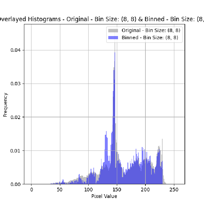
画像のビニング前後の輝度ヒストグラムを正規分布に近似した場合、それぞれの標準偏差は以下のようになります。
- オリジナルの画像: 標準偏差は約41.81
- ビニング後の画像: 標準偏差は約38.09
なぜビニングが重要なのか
ビニングが行われる主な理由は、ノイズの低減と感度の向上です。ノイズとは、画像に含まれるランダムなゴミや粒子のようなもので、これが多いと画像が粗く見えます。感度とは、カメラが光をどれだけ効率よく捉えられるかという指標です。ビニングによって、多くのピクセルが一つにまとめられるので、それぞれの新しいピクセルはより多くの光を捉え、結果としてノイズが減少し、感度が向上します。
ビニングの応用例
ビニングは科学研究からエンターテイメント、産業用途に至るまで幅広い場面で用いられます。例えば、顕微鏡のイメージングでは、ビニングを用いることで暗い場所でも明るい画像を得られます。また、自動車の運転支援システムでは、ビニングが用いられることで夜間や霧の中でもより鮮明な映像が得られ、安全性が向上します。
コメント